BE COMPUTER SCIENCE.

SUBJECT : HIGH PERFORMANCE COMPUTING.

YEAR : MAY 2017

Q1) a) What are the applications of Parallel Computing?

1. i) The parallel computing is suitable for the problems require much more time for computation completion. The several areas in which parallel computing are used usually based on high-end engineering and scientfic problems.
2. ii) This includes computer based simulations and Computational Fluid Dynamics (CFD) as well as other computer based digital image processing and security algorithms.

1. A) Applications of parallel computing in Engineering.

1. i) Parallel computing is used in various engineering problems. These problems typically solved in the form of computer programs in traditional machines.
2. ii) These machines are capable of performing the tasks sequentially but designers closely observed and found the subtasks included in the problem can be performed as different processes simultaneously.

iii) The parallel computations provide the improvements in overall efficiency of the applicatiom. The main factor responsible for efficiency improvements is the speedup of the computations.

1. iv) This phenomenon is adopted in several engineering application domains such as applications of

aerodynamics, optimization algorithms like branch and bound and genetic programming etc.

1. B) Scientfic Applications using Parallel Computing.

1. i) In short scientfic applications are created to show the simulated behaviours of real world entities by using mathematics and mathematical formulas.
2. ii) This means the object exists in the real world are mapped in the form of mathematical models and actions present in that object are simulated using mathematical formula.

iii) Simulations are based on very high-end calculations and require the use of powerful computers. The most of the powerful computers are parallel computers and do the computations in parallel

form.

1. iv) The scientfic applications are major candidates for the parallel computations. For example weather forecasting and climate modeling, Oil exploration and energy research, Drug discovery and genomic research etc. are some of the scientfic applications in which parallel activities are carried out throughout the completion.
2. v) These activities are performed by the tools and techniques provided under the field of parallel computing.

1. C) Commercial Applications Based on Parallel Computing.

1. i) The increasing need for more processing power is full-filled by parallel architectures. The parallel architectures continuously evolve to satisfy the processing requirements of the developing trends of the society.
2. ii) The commercial applications require more processing power in the current market trends because of performing many activities simultaneously.

iii) This creates an inclination towards the use of parallel computing applications for commercial problems. We can consider multimedia applications for commercial problems. We can consider multimedia applications as an example of commercial applications in which parallel computing plays vital role.

1. iv) For large commercial applications such as multimedia applications enhance processing power and most of the circumstances the overall applications should be divided into different modules. These modules work in the close cooperation to complete the overall required task in less amount of time.

1. D) Parallel Computing Applications in Computer Systems.

1. i) In the recent developments in computing the techniques of parallel processing becomes easily adoptable because of growth in computer and communication networks.
2. ii) The computations perform in parallel, by the use of collection of low power computing devices in the form of clusters. In fact a group of computers configured to solve a problem by means of parallel processing is termed as cluster computing systems.

iii) The advances in cluster computing in terms of software frameworks made possible to utilize the computing power of multiple devices for solving of large computing tasks efficiently.

1. iv) The parallel computing is effectively applied in the field of computer security. The internet based parallel computing set-up is suitably used for the implementation of extremely large set of data required for computations.

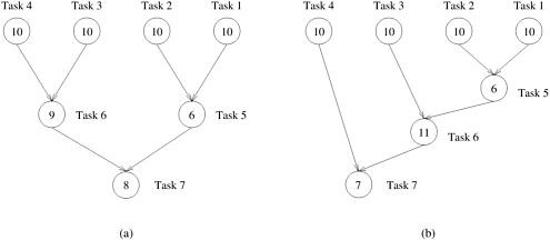
Q1)b) Explain Granuality,Concurrency and Dependency Graph.

1. a) Granuality:

1. i) Granuality is the descriptions about the system in terms of how divisible it is. There are two types of granuality namely fine-granied and course-grained.
2. ii) Fine-grained system has a high granuality. This means in fine-grained, an object is divided into large number of smaller parts.

iii) In the similar ways, course grained refers to the system divided into small number of larger parts. For example, the use of grams to represent weight of an object is more granular than using kilograms to represent weight of the same object.

1. b) Concurrency :

1. i) The tendency of the events in real world to happen at the same time is called as concurrency. The concurrency is one of the natural phenomena in the real world because at a particular instance of the time many things are happening simultaneously. The concurrency is required to deal with for designing the software system for real world problems.
2. ii) There are generally two important aspects when dealing with concurrency for real world problems : ability of dealing and responding external events occur in random order, and required to respond these events in some minimum required interval.

1. c) Dependency Graph :

1. i) It is a directed acyclic graph. Typically a graph is a collection of nodes and edges, the task dependency graph also contains nodes and edges.
2. ii) The nodes in the task-dependency graph represent tasks whereas edges between any two nodes represent dependency between them. For example, there is an edge exists between two nodes T1 and T2, if T2 must be executed after T1.

Q2) a) What are the Principles of Message Passing Programming?

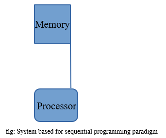
1. i) The message passing paradigm needs some revisions about the conceptual descriptions of the sequential programming paradigm.
2. ii) The fig shows the conceptual view of the machine in which programs execute in sequential fashion. In this approach, a single processor can access the amount of memory available in the machine.

iii) The sequential programming based on the machine in which multiple programs can be allowed to execute by the time-sharing facility provided under the multitasking operating system.

1. iv) There are number of sequential-programming paradigms are considered together for message-passing programming paradigm. In this paradigm, it is required to imagine about the existence of several processors.
2. iv) In this paradigm processors have their own memory elements. The program modules are designed to be executed in each processor.
3. v) The program modules running in different processors need to communicate with each other and the communication takes place by the use of message exchange among modules.

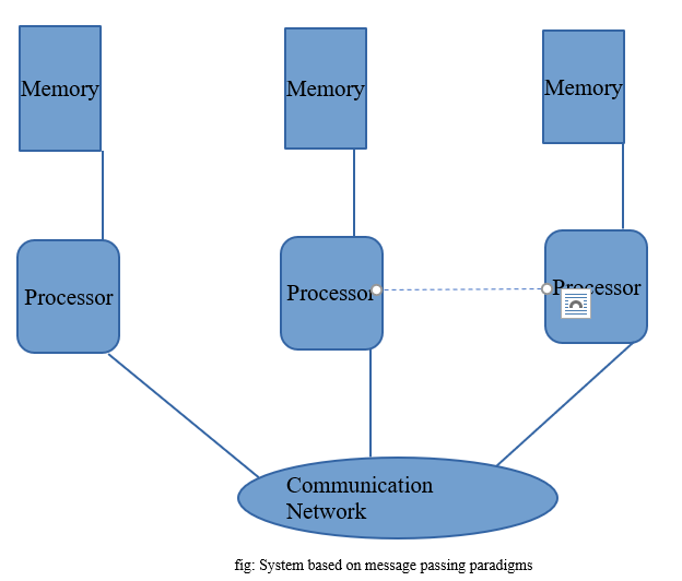
fig: System based on message passing paradigms

1. i) The fig shows the logical view of the machine for message-passing paradigm.
2. ii) The message-passing system does not support sharing of memory by the processors included in the system. This means processors are not allowed to access each other’s memory directly.

iii) The different types of architectures included for the message passing paradigm included for a single processor systems to distributed or shared-memory multiprocessor systems.

1. iv) The message transfer occurs in this paradigm when data movement occurs from one module to another module.
2. v) In this approach the processors involved in the communication need to cooperate with each other to provide information required for the message-transfer.

Q2) b) Explain Non-Blocking communications using MPI.

1. i) The general approach of using the non-blocking communication is the sender and receiver operations do not block involved processes till the completion. The non-blocking send() and receive() primitives return as soon as the process starts.
2. ii) The sender process invokes the send() and instead of waiting for the completion of the send operation it continues with the next task to be performed. The non-blocking nature of the send and receive has advantage in terms of overlapping of computational works.

iii) The non-blocking send returns as soon as possible. It immediately returns control to the calling process as soon as possible so that other parts of the system take control.

1. iv) The send returns immediately and sender continues with other parallel activities and at that period send performs copy operation on the message data.
2. v) The sender process has to verify whether the data has been copied from the send buffer or not. This is handled by the use of send complete Once the data has been copied from the buffer the buffer can be involved in other communication.
3. vi) The MPI system has two functions named as MPI_Isend() and MPI_Irecv() for non-blocking send and receive operations respectively. I in Isend() and Irecv() stands for Initiate.

vii) These functions execute concurrently along with the other computations defined to be performed in the respective programs. At later stages of processing the programs actually involved these functions have to verify about the completion of send and receive operations.

viii) For checking the completion status of Non blocking operations, MPI system has two functions namely MPI_Test() and MPI_Wait().

1. ix) Syntax of MPI_Isend()

int MPI_Isend()

(

void *buffer,

int count,

MPI_Datatype datatype,

int destination,

int tag,

MPI_Comm comm,

MPI_Request *request_handle

)

1. ix) Syntax of MPI_Irecv()

int MPI_Irecv()

(

void *buffer,

int count,

MPI_Datatype datatype,

int source,

int tag,

MPI_Comm comm,

MPI_Request *request_handle

)

Q3) a) Describe Logical Memory Model of a Thread?

Consider the following code segment that computes the product of two dense matrices of size n x n.

1   for (row = 0; row < n; row++)

2       for (column = 0; column < n; column++)

3           c[row][column] =

4               dot_product(get_row(a, row),

5                           get_col(b, col));

The for loop in this code fragment has n2 iterations, each of which can be executed independently. Such an independent sequence of instructions is referred to as a thread. In the example presented above, there are n2 threads, one for each iteration of the for-loop. Since each of these threads can be executed independently of the others, they can be scheduled concurrently on multiple processors. We can transform the above code segment as follows:

1   for (row = 0; row < n; row++)

2       for (column = 0; column < n; column++)

3           c[row][column] =

4               create_thread(dot_product(get_row(a, row),

5                                         get_col(b, col)));

Here, we use a function, create_thread, to provide a mechanism for specifying a C function as a thread. The underlying system can then schedule these threads on multiple processors.

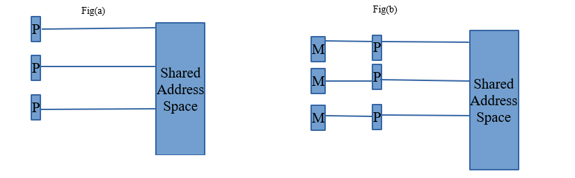
Logical Memory Model of a Thread to execute the code fragment in Example on multiple processors, each processor must have access to matrices a, b, and c. This is accomplished via a shared address space . All memory in the logical machine model of a thread is globally accessible to every thread as illustrated in Figure (a). However, since threads are invoked as function calls, the stack corresponding to the function call is generally treated as being local to the thread. This is due to the liveness considerations of the stack. Since threads are scheduled at runtime (and no apriori schedule of their execution can be safely assumed), it is not possible to determine which stacks are live. Therefore, it is considered poor programming practice to treat stacks (thread-local variables) as global data. This implies a logical machine model illustrated in Figure (b), where memory modules M hold thread-local (stack allocated) data.

While this logical machine model gives the view of an equally accessible address space, physical realizations of this model deviate from this assumption. In distributed shared address space machines such as the Origin 2000, the cost to access a physically local memory may be an order of magnitude less than that of accessing remote memory. Even in architectures where the memory is truly equally accessible to all processors (such as shared bus architectures with global shared memory), the presence of caches with processors skews memory access time. Issues of locality of memory reference become important for extracting performance from such architectures.

Q3) b) Why Synchronization is important? Enlist Thread API’s for Mutex Synchronization.

1. i) Synchronization is the facility provided to the user in almost all programming models used in designing of parallel programs to control the ordering of events on different processors.
2. ii) The parallel executions of some programs depend on the synchronization because without using the synchronization these programs may produce wrong results. The demerit of the synchronization is expensiveness.

Why it is important?

With respect to multithreading, synchronization has the capability to control the access of multiple threads to shared resources. Without synchronization, it is possible for one thread to modify a shared object while another thread is in the process of using or updating that object’s value. This often leads to significant errors.

Thread API’s for Mutex Synchronization.

Thread synchronization is required whenever two threads share a resource or need to be aware of what the other threads in a process are doing. Mutexes are the most simple and primitive object used for the co-operative mutual exclusion required to share and protect resources. One thread owns a mutex by locking it successfully, when another thread tries to lock the mutex, that thread will not be allowed to successfully lock the mutex until the owner unlocks it. The mutex support provides different types and behaviors for mutexes that can be tuned to your application requirements.

The Mutex synchronization APIs are:

• pthread_lock_global_np() (Lock Global Mutex): locks a global mutex provided by the pthreads run-time.
• pthread_mutexattr_destroy() (Destroy Mutex Attributes Object): destroys a mutex attributes object and allows the system to reclaim any resources associated with that mutex attributes object.
• pthread_mutexattr_getkind_np() (Get Mutex Kind Attribute) : retrieves the kind attribute from the mutex attributes object specified by attr.
• pthread_mutexattr_getname_np() (Get Name from Mutex Attributes Object): retrieves the name attribute associated with the mutex attribute specified by attr.
• pthread_mutexattr_getpshared() (Get Process Shared Attribute from Mutex Attributes Object): retrieves the current setting of the process shared attribute from the mutex attributes object.
• pthread_mutexattr_gettype() (Get Mutex Type Attribute) : retrieves the type attribute from the mutex attributes object specified by attr.
• pthread_mutexattr_init() (Initialize Mutex Attributes Object): initializes the mutex attributes object referenced by attr to the default attributes.
• pthread_mutexattr_setkind_np() (Set Mutex Kind Attribute): sets the kind attribute in the mutex attributes object specified by attr.
• pthread_mutexattr_setname_np() (Set Name in Mutex Attributes Object): changes the name attribute associated with the mutex attribute specified by attr.
• pthread_mutexattr_setpshared() (Set Process Shared Attribute in Mutex Attributes Object): sets the current pshared attribute for the mutex attributes object.
• pthread_mutexattr_settype() (Set Mutex Type Attribute) sets the type attribute in the mutex attributes object specified by attr.
• pthread_mutex_destroy() (Destroy Mutex) :destroys the named mutex.
• pthread_mutex_getname_np (Get Name from Mutex) :retrieves the name of the specified mutex.
• pthread_mutex_init() (Initialize Mutex): initializes a mutex with the specified attributes for use.
• pthread_mutex_lock() (Lock Mutex) : acquires ownership of the mutex specified.
• pthread_mutex_setname_np (Set Name in Mutex) : sets the name of the specified mutex.
• pthread_mutex_timedlock_np() (Lock Mutex with Time-Out) : acquires ownership of the mutex specified.
• pthread_mutex_trylock() (Lock Mutex with No Wait) : attempts to acquire ownership of the mutex specified without blocking the calling thread.
• pthread_mutex_unlock() (Unlock Mutex) : unlocks the mutex specified.
• pthread_set_mutexattr_default_np() (Set Default Mutex Attributes Object Kind Attribute) : sets the kind attribute in the default mutex attribute object.
• pthread_unlock_global_np() (Unlock Global Mutex) : unlocks a global mutex provided by the pthreads run-time.

Q4) a) Implement Merge Sort using Synchronization primitives in P-thread.

public void parallelMergeSort() {

synchronized (values) {

if (threadCount <= 1) {

mergeSort(values);

values.notify();

} else if (values.length >= 2) {

// split array in half

int[] left = Arrays.copyOfRange(values, 0, values.length / 2);

int[] right = Arrays.copyOfRange(values, values.length / 2, values.length);

synchronized(left) {

synchronized (right) {

// sort the halves

// mergeSort(left);

// mergeSort(right);

Thread lThread = new Thread(new ParallelMergeSort(left, threadCount / 2));

Thread rThread = new Thread(new ParallelMergeSort(right, threadCount / 2));

lThread.start();

rThread.start();

/*try {

lThread.join();

rThread.join();

} catch (InterruptedException ie) {}*/

try {

left.wait();

right.wait();

} catch (InterruptedException e) {

e.printStackTrace();

}

// merge them back together

merge(left, right, values);

}

}

values.notify();

}

}

}

Q4) b) Illustrate importance of read-write lock for Shared-Address space Model.

1. i) POSIX provides another synchronization tool which is called as read-write locks. Read-Write locks are mainly used to prevent multiple accesses to shared data by more than one thread at a same time. Read-Write lock also provides the facility to distinguish between read lock and write lock which is not supported by mutex.
2. ii) For example when one thread is writing into the shared memory at that time other threads are blocked in mutex i.e. they are not allowed to write into the shared memory. This means at a time, only one thread is allowed to write in mutex. In case of read-write lock multiple threads are allowed to access the data only for reading purpose.

iii)  In shared address space model read-write blocks are mainly important. Consider a situation in which thread 1 wants to write a variable in shared memory and thread 2 wants to read that value of variable that thread 1 has writeen. But before reading the value, thread 3 has updated the value of that variable and after updating, thread 2 has red the value of variable. In this case, thread 2 has red the wrong value. This can result into wrong output because there is no locking mechanism provided. Hence in case of Shared- Address space model, read-write blocks are mainly important.

Q5) a) What are Different Partitioning techniques used in matrix-vector multiplication?

1. i) Vector is a matrix with one column. Here we consider the problem of multiplying a n*n matrix with n*1 matrix which is a vector. Both these matrices are dense. The product is again a vector.
2. ii) Mainly there are two partitioning techniques used in matrix-vector multiplication.
3. a) Row wise 1-D Partitioning.
4. b) Row wise 2-D Partitioning.

1. a) Row wise 1-D Partitioning.
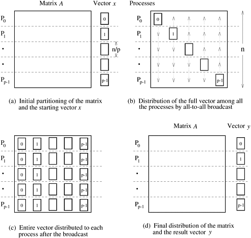
2. i) The first step to multiply matrix and vector is to partition the rows in the matrix into p parts where, p is the number of available processsors. Let us assume that p|n (i.e n mod p = 0).
3. ii) Thus each process Pi where 0<=i<=p-1 gets n/p rows from matrix A and n/p elements from vector B. Fig shows this.

iii) In the next step, by using one to all broadcast, the vector elements allocated to one process is broadcasted to all other processes. Thus each process will now have n/p rows of matrix A and all elements of vector B which are partitioned into p blocks.

Now we will consider two cases where p=n and n>p

where,

p = Number of processes.

n = Number of rows.

Case 1: Number of processes = number of rows i.e. p=n

1. i) In this case each process p_i gets i^th row of matrix A. The process computing i^th element in the resultant vector y by using the following equation.

Complexity of the Algorithm: O(n)

Case 2: Number of processes < number of rows i.e. p < n

In this case, each process gets n/p rows of matrix A. Every process must multiplu these n/p rows with vector x to produce n/p elements of product vector y.

Time Complexity: In this case, type of broadcasting is all to all. All n/p elements of vector X_i  in P_i must be broadcasted to all the remaining processes. This leads to the time complexity of:

t_slog_{p +} t_w(n/p)(p-1)

where,

t_s = message startup time.

t_w = per word transfer time.

1. b) 2-D Partitioning.

Fig 2:

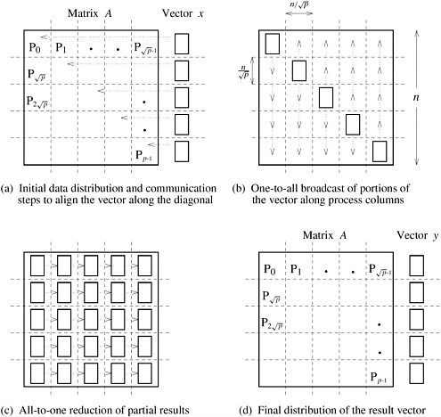
One Element Per Process

We start with the simple case in which an n x n matrix is partitioned among n2 processes such that each process owns a single element. The n x 1 vector x is distributed only in the last column of n processes, each of which owns one element of the vector. Since the algorithm multiplies the elements of the vector x with the corresponding elements in each row of the matrix, the vector must be distributed such that the ith element of the vector is available to the ith element of each row of the matrix. The communication steps for this are shown in Figure 2(a) and (b). Notice the similarity of Figure 1 to Figure 2. Before the multiplication, the elements of the matrix and the vector must be in the same relative locations as in Figure 1(c). However, the vector communication steps differ between various partitioning strategies. With 1-D partitioning, the elements of the vector cross only the horizontal partition-boundaries (Figure 1), but for 2-D partitioning, the vector elements cross both horizontal and vertical partition-boundaries (Figure 2).

As Figure 2(a) shows, the first communication step for the 2-D partitioning aligns the vector x along the principal diagonal of the matrix. Often, the vector is stored along the diagonal instead of the last column, in which case this step is not required. The second step copies the vector elements from each diagonal process to all the processes in the corresponding column. As Figure 2(b) shows, this step consists of n simultaneous one-to-all broadcast operations, one in each column of processes. After these two communication steps, each process multiplies its matrix element with the corresponding element of x. To obtain the result vector y, the products computed for each row must be added, leaving the sums in the last column of processes. Figure 2(c) shows this step, which requires an all-to-one reduction in each row with the last process of the row as the destination. The parallel matrix-vector multiplication is complete after the reduction step.

Parallel Run Time Three basic communication operations are used in this algorithm: one-to-one communication to align the vector along the main diagonal, one-to-all broadcast of each vector element among the n processes of each column, and all-to-one reduction in each row. Each of these operations takes time Q(log n). Since each process performs a single multiplication in constant time, the overall parallel run time of this algorithm is Q(n). The cost (process-time product) is Q(n2 log n); hence, the algorithm is not cost-optimal.

Using Fewer than n2 Processes

A cost-optimal parallel implementation of matrix-vector multiplication with block 2-D partitioning of the matrix can be obtained if the granularity of computation at each process is increased by using fewer than n2 processes.

Consider a logical two-dimensional mesh of p processes in which each process owns an block of the matrix. The vector is distributed in portions of elements in the last process-column only. Figure 2 also illustrates the initial data-mapping and the various communication steps for this case. The entire vector must be distributed on each row of processes before the multiplication can be performed. First, the vector is aligned along the main diagonal. For this, each process in the rightmost column sends its vector elements to the diagonal process in its row. Then a columnwise one-to-all broadcast of these elements takes place. Each process then performs n2/p multiplications and locally adds the sets of products. At the end of this step, as shown in Figure 2(c), each process has partial sums that must be accumulated along each row to obtain the result vector. Hence, the last step of the algorithm is an all-to-one reduction of the values in each row, with the rightmost process of the row as the destination.

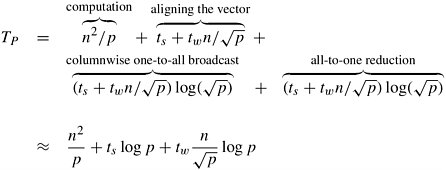
Parallel Run Time The first step of sending a message of size from the rightmost process of a row to the diagonal process (Figure 2(a)) takes time . We can perform the columnwise one-to-all broadcast in at most time by using the procedure. Ignoring the time to perform additions, the final rowwise all-to-one reduction also takes the same amount of time. Assuming that a multiplication and addition pair takes unit time, each process spends approximately n2/p time in computation. Thus, the parallel run time for this procedure is as follows:

Equation 8.7

Scalability Analysis By using Equations 8.1 and 8.7, and applying the relation To = pTp – W (Equation 5.1), we get the following expression for the overhead function of this parallel algorithm:

Equation 8.8

We now perform an approximate isoefficiency analysis along the lines of Section 5.4.2 by considering the terms of the overhead function one at a time (see Problem 8.4 for a more precise isoefficiency analysis). For the ts term of the overhead function, Equation 5.14 yields

Equation 8.9

Equation 8.9 gives the isoefficiency term with respect to the message startup time. We can obtain the isoefficiency function due to tw by balancing the term log p with the problem size n2. Using the isoefficiency relation of Equation 5.14, we get the following:

Equation 8.10

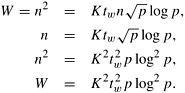
Finally, considering that the degree of concurrency of 2-D partitioning is n2 (that is, a maximum of n2 processes can be used), we arrive at the following relation:

Equation 8.11

Among Equations 8.9, 8.10, and 8.11, the one with the largest right-hand side expression determines the overall isoefficiency function of this parallel algorithm. To simplify the analysis, we ignore the impact of the constants and consider only the asymptotic rate of the growth of problem size that is necessary to maintain constant efficiency. The asymptotic isoefficiency term due to tw (Equation 8.10) clearly dominates the ones due to ts (Equation 8.9) and due to concurrency (Equation 8.11). Therefore, the overall asymptotic isoefficiency function is given by Q(p log2 p).

The isoefficiency function also determines the criterion for cost-optimality . With an isoefficiency function of Q(p log2 p), the maximum number of processes that can be used cost-optimally for a given problem size W is determined by the following relations:

Equation 8.12

Ignoring the lower-order terms,

Substituting log n for log p in Equation 8.12,

Equation 8.13

The right-hand side of Equation 8.13 gives an asymptotic upper bound on the number of processes that can be used cost-optimally for an n x n matrix-vector multiplication with a 2-D partitioning of the matrix.

Q5) b) Describe Cannon’s Algorithm for matrix multiplication with suitable example.

1. i) Cannon’s algorithm works in similar fashion as simple parallel algorithm. But it is more memory efficient.
2. ii) In simple parallel algorithm, blocks A and B were broadcasted through rows and columns. In Cannon’s Algorithm, instead of broadcasting the blocks are shifted. See the following figure in which blocks of A are shifted row wise and blocks of B are shifted column wise.

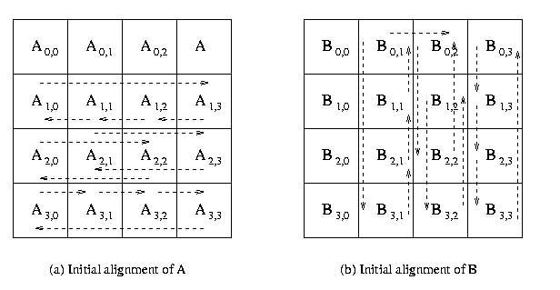
iii) While assigning the blocks to the processes, the row i of blocks in A are shifted i blocks and column i of blocks in A are shifted i blocks.

1. iv) After initial the initial allotment to the processes, the process P _i,j modifies blocks A_x,y and B_y,z . It will find the partial result by multiplying both blocks.
2. v) After first shift, the process P_i,j has A_x,(y+1) mod p^1/2  and B_(x+1)  mod p^1/2 ,y. Now multiply these blocks and add result to C_i,j.
3. vi) This process is repeated p^1/2 Shown in the following figure.

vii) The time complexity of cannon’s algorithm is n³/p + t_slog p + 2t_wn³/p^1/2  which is same as simple parallel algorithm. But the main advantage of cannon’s algorithm over simple parallel is memory efficiency hence in case of space complexity at any given time, a process stores one block of A and one block of B and in case of simple parallel alogorithm each process has to save p^1/2 blocks of A and p^1/2  blocks of B. Hence Cannon’s is memory efficient.

Q6) a) Describe Different techniques of latency hiding.

1. i) Generally the higher latency is due to the shared resources in a network, that too shared memory. The following methods can be used to hide the latency.
2. a) Perfecting Instructions.
3. b) Use of coherant cache.
4. c) Use of relaxed memory consistency model.
5. d) Communication.

1. a) Perfecting Instructions.
2. i) The instructions that are to be executed in next clock cycles are perfected. This can be either hardware of software controlled.
3. ii) The hardware controlled perfecting is achieved by using long cache lines or instruction look ahead. Software controlled perfecting executes the perfecting instructions explicitely to move data close to the processor before it is needed.

b)Use of Coherant Cache.

1. i) Multiple caches are used to store the data. The cache coherance has two levels.
2. Every write operation occurs instantaneously.
3. All processor present in the network see the same sequence of changes in the data.
4. ii) The cache coherenace is mainly used to manage the conflicts between the cache and main memory. The access to cache memory is faster than main memory. This reduces / hides the latency in case of fetching any instruction or data.

1. c) Use of relaxed memory consistency model.
2. i) In relexed or release model, the synchronization accessor of data in the program are idenfified. They are classified as locks or unlocks. This provides flexibility and fast access.
3. ii) In multiprocessor architecture, relaxed memory model is implemented by buffering the write operations and allowing the read operations.

1. d) Communication.
2. i) In case of communication, a block of data is transferred rather than a single data; Generating a communication before it is actually needed helps to reduce the latency. This is known as pre-communication.

Q6) b) How latency hiding is different than latency reduction?

Memory Latency Hiding: Finding something else to do while waiting for memory.

Memory Latency Reduction: Reducing time operations must wait for memory.

Latency Hiding in Covered Architectures:

1. Superscalar (Hiding cache miss.)
2. While waiting execute other instructions.
3. Can only cover part of miss latency.

2. Multithreaded
3. While waiting execute other threads.
4. Can cover full latency.

iii. Requires effort to parallelize code.

1. Parallel code possibly less efficient.

3. Multiprocessor
4. Latency problem worse due to coherence hardware and distributed memory.

Memory Latency Reduction Approaches

1. Vector Processors
2. ISA and hardware eciently access regularly arranged data.

ii.Commercially available for many years.

2. Software Prefetch
3. Compiler or programmer fetch data in advance.
4. Available in some ISAs.

3. Hardware Prefetch
4. Hardware fetches data in advance by guessing access patterns.

4. Integrated Processor /DRAM

i.Reduce latency by placing processor and memory on same chip.

5. Active Messages

i.Send operations to where data is located.

Q7) a) Write a Short note on (any two)

1. Parallel Depth First Search.
2. Search Overhead factor
3. Power aware Processing.

1. Parallel Depth First Search.
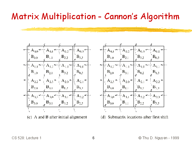
2. i) To solve a discrete optimization problem, depth first search is used if it can be formulated as tree search problem. Depth-first search can be performed in parallel by partitioning the search space into many small, disjunct parts (subtrees) that can be explored concurrently. DFS starts with initial node by generating its successors.
3. ii) If any node has no successors, then it indicates that there is no solution in that path. Thus backtracking is done and continued to expand another node. Following figure gives the DFS expansion of the 8-puzzle.

iii) The initial configuration is given in (A) .There are only two possible moves,Blank up or blank right. Thus from (A) two children or successors are generated. Those are (B) and (C).

1. iv) This is done in step 1. In step 2, any one of (B) and (C) is selected. If (B) is selected then its successors (D), (E) and (F) are generated. If (C) is selected then its successors (G), (H) and (I) are generated.
2. v) Assuming (B) is selected, and then in the next step (D) is selected. It is clear that (D) is same as (A), thus backtracking is necessary. This process is repeated until the required result is found.

2. Search Overhead Factor.

Parallel search algorithms incur overhead from several sources. These include communication overhead, idle time due to load imbalance, and contention for shared data structures. Thus, if both the sequential and parallel formulations of an algorithm do the same amount of work, the speedup of parallel search on p processors is less than p. However, the amount of work done by a parallel formulation is often different from that done by the corresponding sequential formulation because they may explore different parts of the search space.

Let W be the amount of work done by a single processor, and Wp be the total amount of work done by p processors. The search overhead factor of the parallel system is defined as the ratio of the work done by the parallel formulation to that done by the sequential formulation, or Wp/W. Thus, the upper bound on speedup for the parallel system is given by p x(W/Wp). The actual speedup, however, may be less due to other parallel processing overhead. In most parallel search algorithms, the search overhead factor is greater than one. However, in some cases, it may be less than one, leading to superlinear speedup. If the search overhead factor is less than one on the average, then it indicates that the serial search algorithm is not the fastest algorithm for solving the problem.

To simplify our presentation and analysis, we assume that the time to expand each node is the same, and W and Wp are the number of nodes expanded by the serial and the parallel formulations, respectively. If the time for each expansion is tc, then the sequential run time is given by TS = tcW. In the remainder of the chapter, we assume that tc = 1. Hence, the problem size W and the serial run time TS become the same.

3. Power aware Processing.
4. i) In high-performance systems, power-aware design techniques aim to maximize performance under power dissipation and power consumption constraints. Along with thsi, the low-power design techniques try to reduce power or energy consumption in portable equipment to meet a desired performance. All the power a system consumes eventually dissipates and transforms into heat.
5. ii) The power dissipation and related thermal.

Q7) b) Elucidate Thread Organization in Detail.

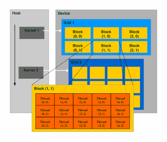
A thread block is a programming abstraction that represents a group of threads that can be executing serially or in parallel. For better process and data mapping, threads are grouped into thread blocks. The number of threads varies with available shared memory. The number of threads in a thread block is also limited by the architecture to a total of 512 threads per block. The threads in the same thread block run on the same stream processor. Threads in the same block can communicate with each other via shared memory, barrier synchronization or other synchronization primitives such as atomic operations.Multiple blocks are combined to form a grid. All the blocks in the same grid contain the same number of threads. Since the number of threads in a block is limited to 512, grids can be used for computations that require a large number of thread blocks to operate in parallel.CUDA is a parallel computing platform and programming model that higher level languages can use to exploit parallelism. In CUDA, the kernel is executed with the aid of threads. The thread is an abstract entity that represents the execution of the kernel. A kernel is a small program or a function. Multi threaded applications use many such threads that are running at the same time, to organize parallel computation. Every thread has an index, which is used for calculating memory address locations and also for taking control decisions.

Q8) a) Write Short notes on

1. Distributed Memory.
2. Optical Computing.
3. Green Computing.

1. Distributed Memory.
2. i) In computer science, distributed memory refers to a multiprocessor computer system in which each processor has its own private memory. Computational tasks can only operate on local data, and if remote data is required, the computational task must communicate with one or more remote processors.
3. ii) In contrast, a shared memory multiprocessor offers a single memory space used by all processors. Processors do not have to be aware where data resides, except that there may be performance penalties, and that race conditions are to be avoided.In a distributed memory system there is typically a processor, a memory, and some form of interconnection that allows programs on each processor to interact with each other.

iii) The interconnect can be organised with point to point links or separate hardware can provide a switching network. The network topology is a key factor in determining how the multiprocessor machine scales. The links between nodes can be implemented using some standard network protocol (for example Ethernet), using bespoke network links (used in for example the Transputer), or using dual-ported memories.

2. Optical Computing.
3. i) Optical or photonic computing uses photons produced by lasers or diodes for computation. For decades, photons have promised to allow a higher bandwidth than the electrons used in conventional computers.
4. ii) Most research projects focus on replacing current computer components with optical equivalents, resulting in an optical digital computer system processing binary data. This approach appears to offer the best short-term prospects for commercial optical computing, since optical components could be integrated into traditional computers to produce an optical-electronic hybrid. However, opto electronic devices lose 30% of their energy converting electronic energy into photons and back; this conversion also slows the transmission of messages. All-optical computers eliminate the need for optical-electrical-optical (OEO) conversions, thus lessening the need for electrical power.

iii) Application-specific devices, such as synthetic aperture radar (SAR) and optical correlators, have been designed to use the principles of optical computing. Correlators can be used, for example, to detect and track objects, and to classify serial time-domain optical data.[

3. Green Computing
4. i) Green computing is the environmentally responsible and eco-friendly use of computers and their resources. In broader terms, it is also defined as the study of designing, manufacturing/engineering, using and disposing of computing devices in a way that reduces their environmental impact.
5. ii) Green computing, green ICT as per International Federation of Global & Green ICT “IFGICT”, green IT, or ICT sustainability, is the study and practice of environmentally sustainable computing or IT.

iii) The goals of green computing are similar to green chemistry: reduce the use of hazardous materials, maximize energy efficiency during the product’s lifetime, the recyclability or biodegradability of defunct products and factory waste. Green computing is important for all classes of systems, ranging from handheld systems to large-scale data centers.

1. iv) Many corporate IT departments have green computing initiatives to reduce the environmental effect of their IT operations.

Q8) b) Intricate Sorting Issues in Parallel Computers.

1. i) The major task in the Parallel Algorithms is to Distribute the elements to be sorted onto the available processes. Following are the issues that are to be addressed while distributing.

1 .Where the input and output sequences are stored.

1. i) In case of parallel algorithm, the data may be present in one process or may be it is distributed throughout the processes. Wherever sorting is a part of any other algorithm, it is better to distribute the data among processes.
2. ii) To distribute the sorted output sequence among the processes, the processes must be enumerated. This enumeration is used to specify the order of the data.

iii) For example, the Process P1 comes before Process P2 in enumeration, then all the elements in Process P1 comes before all the elements in Process P2 in the sorted sequence.

1. iv) This enumeration mainly depends on the tyoe on interconnection network.

2. How Comparisons are Performed.
3. i) In case of sequential algorimths, all the data that is to be compared is present on only one process, whereas in case of parallel algorithms, data is distributed to n number of processes. Hence there can be two cases in case of how comparisons are performed.

Case 1: Each Process Has Only One Element

2. i) Let Process P1 contains element having value ‘1’ and Process P2 contains element having value as ‘2’. Let process P1 comes before P2. To arrange two elements in ascending order, first thing to do is send the element from one process to another and compare them in the process.
3. ii) Here P1 keeps smaller value whereas P2 keeps larger.

Iii) Hence both the process send the data to one another. So both the process can perform compare operation.

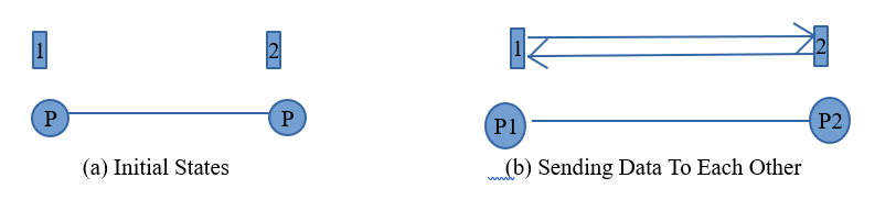
2. iv) Process P1 and P2 both contains value 1 and 2 after sending Data to each other. Now because of enumeration, Process P1 comes before Process P2. Hence Process P1 Performs min(1,2) compare operation i.e. Minimum between two elements gets selected. In this case it is 1.
3. v) Similiarily, Process P2 performs max(1,2) compare opertion i.e. Maximum between two elements is selected.In this case it is 2.

1. v) If P1 and P2 are neighbours in the interconnection network and communication is bidirectional, then communication cost is ts + tw.

Case 2: Each Process Has More Than one Element.

1. i) When there is large sequence is to be sorted and number of processes available in less then each process stores more than one element in its memory. If there are n elements to be sorted and number of processes available is p, then n/p elements are allotted to each process.
2. ii) In this case also, consider the example of two processes P1 and P2. Let us consider that P1 contains elements (2,5,8,9) and P2 contains (1,3,6,7).

iii) Similar to Case 1, in this case also both the processes sends the data to each other using communication network.

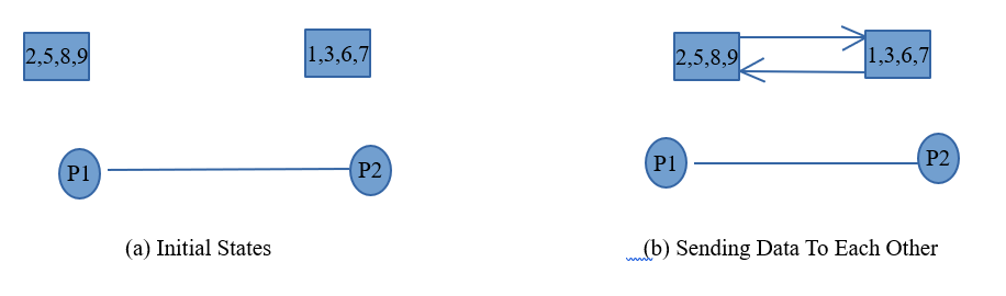
1. iv) Again Both the process have all the data of each other similar to case 1.
2. v) On next step Data is sorted and again minimum and maximum operations are performed. Minimum half is kept in P1 and Maximum in P2.
3. vi) After that two process are merged to get output.

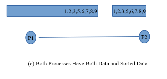
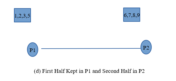
vii) Complexity: O(ts + tw n/p).

n/p since each process contains n/p and communication is bidirectional.